Machine learning to recreate the active matter phase diagram

· 06 Mar 2021

Machine learning has become a powerful tool to aid in the characterization of materials.$^{1-4}$ In this post I will talk about how it can be used to characterize a specific type of material, active matter. As it turns out, active matter systems can spontaneously separate into dense and dilute phases, strictly due to their activity, through a process called motility-induced phase separation (MIPS). What makes this so intriguing is that we can observe this phase separation without any attractive interactions to bring particles together! This means that activity can—under the right conditions—create attraction between particles resulting in this separation. In this post I will discuss my efforts to help characterize this behavior using machine learning. The full paper is currently available on arXiv as Machine Learning for Phase Behavior in Active Matter and code to reproduce the results is available here. The remainder of the post will be outlined as follows:

What is active matter?
Basics of phase behavior.
Using ML to predict phase behavior.
Prediction

What is active matter?

Active matter is a type of material in which each constituent is self-propelled (i.e. a swarm of bacteria, flock of birds, or school of fish). These materials can exhibit unique collective and emergent behavior purely due to their activity, which is dramatically different from their passive counterparts.

Starlings

While each example I have given has been in a biological context, there are synthetic active materials as well. The Janus particle—named after the two-faced Roman god, Janus—is a polystyrene bead with one hemisphere coated in a catalytic material like platinum is a common example.

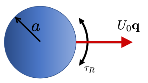
A common model for studying active matter is the active Brownian particle (ABP) model. In this model we reduce each active particle to a sphere of radius $a$ that swims in direction $\mathbf{q}$ at speed $U_{0}$ and reorients itself on a timescale $\tau_{R}$. The origin of the interesting phenomena exhibited by these systems is the nature of their active motion. Each particle swims in its direction for a time $\tau_{R}$ before it reorients and swims in a new direction, resulting in a directed motion with a persistence length $\ell = U_{0}\tau_{R}$. We can get a sense for how strong this persistence is by looking at how far a particle swims before reorienting ($\ell$) relative to its body size ($a$). This results in the dimensionless parameter $Pe_{R} \equiv a / \ell$, the reorientation Péclet number. This parameter will be important later! Now, we have our model which accounts for a swimming motion and a stochastic torque that results in reorientions. Next, I will discuss phase behavior in a general context. (These details are simply to give a broader context to the issue at hand, but are not specifically required to understand the gist of this post.)

Basics of phase behavior.

Phase behavior broadly refers to how a material changes its state of matter and the complex interactions between these distinct states (phases). The phases that we are all most familiar with include solids, liquids, and vapors. There are more nuanced states of matter such as gels, crystals, and plasmas, but we will focus on liquids and vapors. In order to understand phase behavior we would typically rely on thermodynamics, which is the branch of science that deals with the relationship between heat and other forms of energy and how it affects physical properties of matter.

Different phases of a material have distinct properties (like the change in density between liquid water and steam). If we have a material at a specific temperature and pressure, we can determine it’s phase by minimizing its free energy. Normally the free energy minimum exists in one discrete phase. However, two or more phases can coexist if they are in mechanical, thermal, and chemical equilibrium. That is the pressure $P$, temperature $T$, and chemical potential $\mu$ of each phase are equal. A phase diagram, like in the picture above, simply shows where different phases coexist (i.e. the interfaces between the phase regions). Let’s now talk about how machine learning fits into this problem.

Using ML to predict phase behavior.

Active materials are different from “passive” materials because their activity drive them far from equilibrium. This means we can’t use the thermodynamic frameworks that we would normally use to characterize phase behavior in traditional materials because things like temperature are ill-defined (for those interested, we can’t rely on equipartition theorem to relate the kinetic energy to temperature because we don’t have a well-defined Hamiltonian).

We can still use mechanics! Quantities such as the pressure $P$ and packing fraction $\phi \equiv n \pi a^{2}$ (in two spatial dimensions), where $n$ is the number density of particles, are still well-defined. Using these quantities and our ABP model, we could numerically recreate the phase diagram by running simulations over different combinations of packing fraction ($\phi$) and activity ($Pe_{R}$), computing the pressure, and determining phase transitions from mechanical instabilities. What’s the drawback?

While simulating every point on phase space is possible and reliable, it quickly becomes prohibitively expensive from a computational standpoint. That is where machine learning comes in. If I can use multiple particle properties to predict the phase behavior, then we can forego performing a large number of expensive simulations.

Problem Setup

My goal was to provide phase labels, dense (liquid) or dilute (gas), for each particle at a given point in phase space at a specific time. To do this I took a combination of per-particle features—local density, number of neighbors, speed, etc.—and used these to train a deep neural network to predict particle phase. Something similar was done for Lennard-Jones fluids by Ha et. al, so it seemed like a reasonable approach.

From simulations, I knew where the critical point (onset of phase separation) was and used data above this point (on the $Pe_{R}–\phi$ plane) as my training data. Interestingly, active systems have much larger fluctuations than passive systems. This effect is compounded as we approach the critical point. As a system gets close to undergoing a transition like the liquid–vapor transition, density fluctuations grow because particles are on the verge of splitting into two phases with distinct densities. These fluctuations actually become quite difficult to handle using just single-particle properties. Therefore, to remedy this I decided to incorporate structural data into the system by using a graph convolutional neural network (GNN).

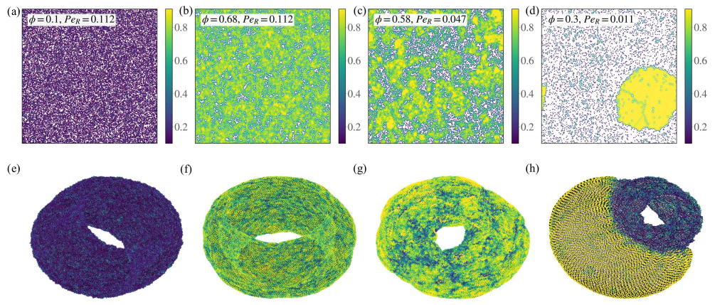
I could have used a convolutional neural network (CNN) to incorporate spatial-relationships into my learning problem, but that would require I introduce an additional lengthscale into the problem. To use a CNN, I would have to discretize space in some way because particles aren’t laid on a grid like pixels, but are instead amorphous. However, using a GNN doesn’t require that my particles be on a rectilinear grid, and I can use more meaningful methods to draw connections. Thus, I used particle neighbors (specifically Voronoi neighbors) to make connections between particles and represent a snapshot of the system as a graph. Now, I can use information from my local environment to influence my predictions. Snapshots from simulations (top) with their graph representations (bottom) are shown below. Here the color is based on the local (Voronoi) density. From the graph structure alone we can see distinct differences depending on the phase that the system is in, whether it be dilute, dense, near the critical point, or strongly phase-separated (moving from left to right in the picture).

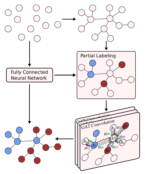
Incorporation of the graph structure resulted in my final learning scheme. First I used a dense neural network to get softmax probabilities for particles in a system. Then, I represent the system as a graph, where each node is a particle, and label those that were confidently predicted (>80% probability) by the deep neural network. This results in a semi-supervised learning problem for the GNN. The partially labeled graph and feature data are then fed into my GNN, which is comprised of 3 GAT layers. Finally, the initial and GNN predictions are averaged to get the final particle labels. A schematic of this process is in the picture below.

Prediction

With the model set, I was able to predict particle phase at different points in the phase diagram. Since phase is a macroscopic idea, I found it more interesting to look at a point in phase space and perform an ensemble average over all particle labels to determine if that point in phase space was in the dense, dilute, or coexistence region of the phase diagram. I then average this prediction across 6 instances in time to account for instantaneous fluctuations.

Active Matter Phase Diagram

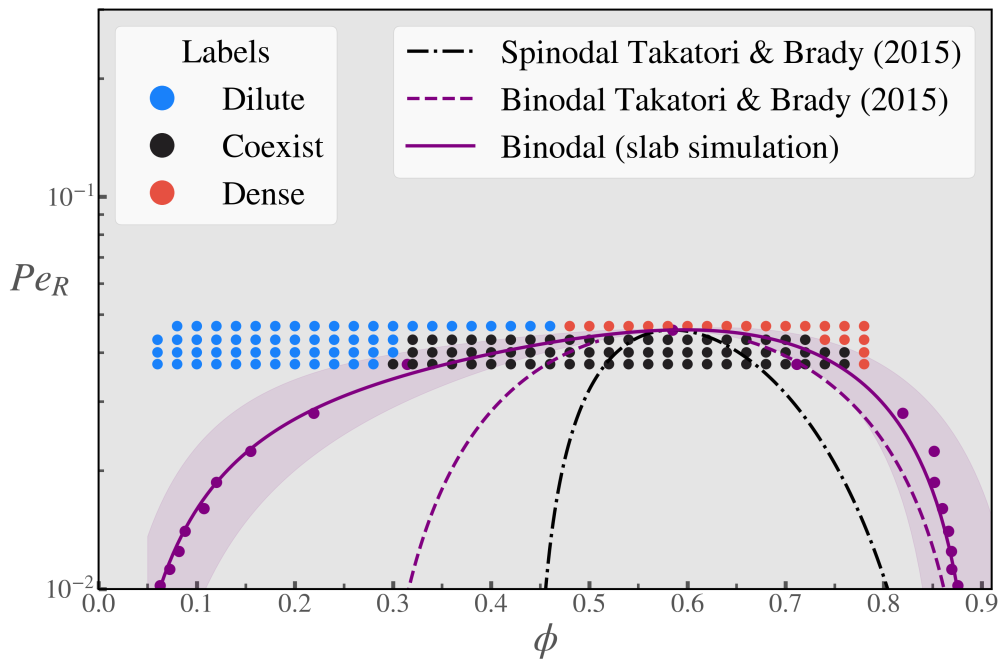
This turns out to work really well! Here I show individual simulation points with their labels and compare them to some previous theoretical works (the dashed lines). The purple points and solid purple line are the ground truth for the coexistence line (binodal) from the simulations. Thanks to this ML method, I was able to recreate the phase diagram using less than 10 data points for each ($Pe_{R}$,$\phi$) pair, as opposed to needing thousands of them to get an accurate measure of the coexistence line via simulation. Also, through this method I gained a lot of insights into what is important for phase separation in ABPs and what my model was learning because the features have physical meaning.

This was an exciting problem to work on and resulted in a lot of future work. Thank you for reading! As mentioned at the top, this work can be found on arXiv as Machine Learning for Phase Behavior in Active Matter and code to reproduce the results is available here.

References

- J. Carrasquilla and R. G. Melko, “Machine learning phases of matter,” Nature Physics 13, 431–434 (2017).
- E. P. L. van Nieuwenburg, Y.-H. Liu, and S. D. Huber, “Learning phase transitions by confusion,” Nature Physics 13, 435–439 (2017).
- P. Suchsland and S. Wessel, “Parameter diagnostics of phases and phase transition learning by neural networks,” Physical Review B 97, 174435 (2018).
- K. Swanson, S. Trivedi, J. Lequieu, K. Swanson, and R. Kondor, “Deep learning for automated classification and characterization of amorphous materials,” Soft Matter 16, 435–446 (2020).